Solving the WDF 2025 Scheduling Challenge: A Three-Week Journey

In early 2025, my teammates Gaël Garnier, Augustin Logeais and I found ourselves staring at a problem that looked deceptively simple on paper. The West Data Festival AI Challenge, organized by ESIEA and Luminess, asked us to schedule factory workers across a production pipeline. Three weeks later, our solution would outperform the baseline by 48%, but that number doesn't capture the real story. It doesn't capture the Discord calls at 2 AM, the subtle bug that nearly broke our final submission, or the moment we realized that sometimes the best way forward is to combine two seemingly incompatible approaches.

The problem that wasn't just a schedule

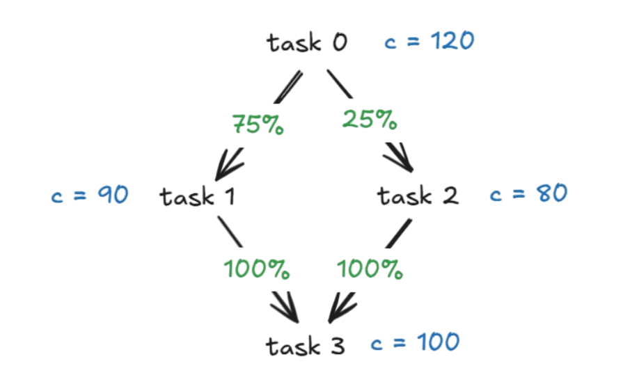
The challenge presented itself as a scheduling problem, but it quickly revealed layers of complexity that made classical job-shop scheduling look quaint. We were given production scenarios, each defined by a set of tasks, operators, and discrete time slots. The tasks formed a directed acyclic graph, where each node represented a production step and edges carried percentages dictating how intermediate outputs flowed between them.

Task 0 had infinite raw materials. Task 3 (or 4, or 12, depending on the instance) produced the finished goods we were judged on. Everything in between was a delicate dance of flow conservation.

An operator working on task in time slot could process up to units, but only if enough input had accumulated from all predecessor tasks. The DAG edges carried percentages: if task A fed 75% into task B, then B could receive at most units from A for every unit A produced.

This wasn't just about assigning tasks to operators. We had to respect real-world constraints that made every decision ripple through the timeline. Operators had shift windows. They could only work on one task per slot. Certain operator-task pairs were incompatible. When an operator started a task, they had to continue for a minimum number of consecutive slots (no one-slot sessions), but couldn't exceed a maximum without switching. Each operator needed a minimum total workload, but also couldn't spend too many slots on any single task.

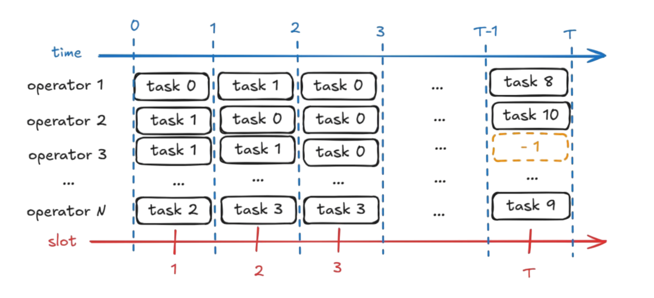
A valid schedule was essentially a matrix: operators as rows, time slots as columns, each cell containing a task ID or -1 for idle. The score was the total output from final tasks. Simple to state, but the search space grew combinatorially with each added constraint.

Exact methods meet reality

In our first week, we did what any good engineering students would do: we tried to solve it exactly. We built a MILP formulation using PuLP, defining binary variables for whether operator performs task at time . The constraints translated cleanly: shift windows, one-task-per-slot, session lengths. The objective maximized final task output.

For tiny instances (4 tasks, 2 operators, 24 slots), CBC found the optimal solution in about 18 seconds. But when we scaled to 4 tasks and 96 slots, the solver ran for minutes without finishing. The model ballooned to thousands of binary variables, and the inter-slot flow constraints created a dense constraint matrix that choked the branch-and-bound tree.

We hit the classic wall: exact methods give guarantees, but only if they finish. Our competition instances went up to 100 tasks and 240 slots. A pure MILP approach would need days, not minutes.

That's when we started talking about hybrid approaches. Not as a compromise, but as a synergy. What if we could get the best of both worlds: the global exploration of heuristics and the local optimality guarantees of exact methods?

Hybrid insight

The breakthrough came during one of those late Discord sessions. We were sketching out a simulated annealing framework while grappling with MILP scaling, and the idea emerged naturally: why not run MILP on small windows instead of the whole thing?

Our simulated annealing would maintain a complete schedule, making moves like swapping task blocks between operators or shifting timelines. Every few thousand iterations, we'd pause and extract a time window (say, 24 consecutive slots for all operators). We'd feed this subproblem to CPLEX as a MILP, letting it find the optimal assignment for that window while keeping everything else fixed. Then we'd splice the optimized window back into the full schedule and continue annealing.

This did two things. First, it kept the MILP tractable: a 24-slot window for 5 operators might have a few hundred variables, solvable within 60 seconds. Second, it gave the annealing a periodic "intensification" step that pure local search couldn't achieve. The metaheuristic explored the global space, while MILP polished the local details to provable optimality.

We paired this with a greedy initialization that scheduled tasks in topological order, spreading them in "bands" across the timeline. Task 0 would occupy early slots across many operators, feeding intermediate tasks that would be scheduled later. This gave us a valid starting point that wasn't random noise.

The neighbor moves we designed were specific to the problem's structure: reassigning contiguous blocks, swapping operator schedules for a period, or focusing on bottleneck tasks identified by analyzing the DAG's critical path. Each move was immediately validated against all constraints. If a move broke a min-session rule, we'd either extend the session or reject the move entirely. This kept our search in the feasible space, which was crucial given how tightly constrained the problem was.

Scaling up (Google Cloud)

By week two, we had a working hybrid solver that scored 1.1x the baseline. The professor overseeing the competition, Manuel Clergue, sent us a Teams message:

That message arrived at the perfect time. We were exhausted, debugging subtle issues in our flow simulation. One particularly nasty bug had the MILP allowing tasks to consume output from predecessor tasks in the same time slot, while our simulation correctly required a one-slot delay. We spotted this by comparing MILP solutions against our validator. The fix involved adding constraints to enforce this delay, aligning the MILP's optimistic view with reality.

But we had a new problem: computation time. Our laptops would heat up and throttle during long runs. The free academic license for IBM CPLEX gave us a powerful solver, but not powerful hardware.

We turned to Google Cloud Platform's free tier. We spun up a C2D Standard VM with an AMD EPYC processor, giving us multiple fast cores and enough memory to run CPLEX with parallel threads. The workflow became: test locally on small instances, then deploy overnight to GCP for the full batch of 30 competition instances. What took an hour on a laptop finished in 15 minutes on the cloud VM.

This changed our iteration cycle. We could test parameter tweaks (annealing cooling rates, MILP window sizes, frequency of intensification steps) and get results by morning. The spreadsheet we maintained to track scores for each instance became our compass. We could see patterns: pure MILP solved the smallest instances optimally, the hybrid approach dominated medium ones, and our annealing with infrequent MILP calls worked best for the largest cases.

Grind and edge cases

The final week was a blur of optimization and edge-case hunting. We implemented a dynamic reheating scheme for the simulated annealing: if the score plateaued for too long, we'd spike the temperature to escape local optima. We hunted down off-by-one errors in the min-work-slots constraint, the kind of bug that only appears when an operator's schedule ends exactly one slot short of the requirement.

We also focused on window selection strategy. Instead of optimizing arbitrary 24-slot blocks, we started targeting windows containing the most critical tasks. We'd analyze the DAG to identify bottlenecks (tasks with high capacity but limited operator availability, or nodes that multiple paths converged on) and prioritize MILP windows that contained these tasks. This made each intensification step more impactful.

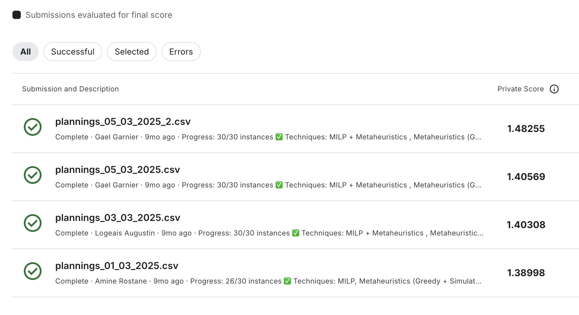
Our performance tracking spreadsheet guided the final ensemble strategy. We built multiple solver variants and, for each instance, automatically routed it to the variant that historically performed best. This wasn't against the rules; the competition allowed any approach per instance. It gave us a final boost that pushed our average score from 1.35 to 1.48.

Final hours

The night before the deadline, we ran our solver one last time on all 30 instances with our best-discovered settings. The GCP VM hummed through the computations while we triple-checked the output schedules with our validator. No invalid schedules could slip through; the platform would reject the entire submission if even one constraint was violated.

At 3 AM, the final CSV was ready. We submitted. The leaderboard updated. Score: 1.48. We had won by a comfortable margin.

What worked and what we learned

Looking back, several things made this project click. First, we invested heavily in understanding the problem. Building our own validator and simulator gave us intuition that guided every decision. When you see idle operators or starved bottleneck tasks in simulation, the fixes become obvious.

Second, the hybrid strategy wasn't just a technical choice; it was a philosophical one. Exact methods and heuristics are often presented as alternatives, but they complement each other beautifully. MILP alone would never finish. Simulated annealing alone might wander aimlessly. Together, they covered each other's weaknesses.

Third, resourcefulness mattered. Academic licenses and cloud free tiers gave us access to industrial-grade tools. You don't need a massive research budget to tackle hard problems; you need to know what's available and how to use it efficiently.

Finally, the teamwork. Our Discord channel was equal parts code repository, debugging war room, and morale booster. When one of us got stuck, another had the key insight. We each brought slightly different strengths, and this complementarity saved us time. The whole was greater than the sum of its parts.

Three weeks, many late nights, and a 1.48 score later, we had not just won a competition. We had experienced the full arc of research and development, from confused initial sketches to a solution that the organizers said might inform real industrial planning tools. The theories we learned in class, from branch-and-bound to Markov chains, weren't just academic exercises. They were tools that, when combined with persistence and collaboration, could solve problems that mattered.

For me and my teammates, that realization was worth more than any score.

Special thanks

• Manuel Clergue (Professor)
• Gaël Garnier (Teammate)
• Augustin Logeais (Teammate)
• Tony Bonnet (Luminess Engineer)
• Arthur Moulinier (Luminess Engineer)
• Samuel Ansel (Luminess Engineer)